| Channel | Publish Date | Thumbnail & View Count | Download Video |
|---|---|---|---|
 | Publish Date not found | 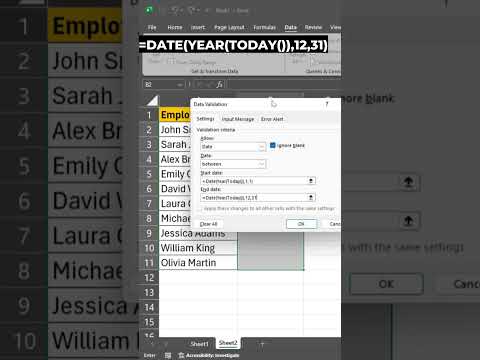 0 Views |
Step 1: Select cell
Click the cell: First, click the cell or range to which you want to apply this rule.
Step 2: Open data validation
Go to the Data tab:
Find and click the Data tab on the ribbon at the top of Excel.
In the Data Tools group, locate and click Data Validation.
Step 3: Define validation criteria
Select date validation:
On the Settings tab, go to the Allow drop-down menu and select Date.
Next, set the data criteria to “Between.”
For the start date, enter the formula: =DATE(YEAR(TODAY()),1,1). This means January 1 of the current year.
For the end date, enter =DATE(YEAR(TODAY()),12,31), which means December 31 of the current year.
Step 4: Add a custom input message
Go to the Enter Message tab:
Click the Enter Message tab.
Select the Show input message when cell is selected check box.
#ExcelHacks #DateValidation #ExcelTips #ExcelTricks #DataManagement #YearSpecificValidation #PreventOldDates #ExcelTutorial #DataAccuracy #excelmagictrick
Please take the opportunity to connect with your friends and family and share this video with them if you find it useful.